Lab 5
Number Detection Using ML
Abstract: We found this week’s lab quite interesting. We did not manage to make the suggested solution work—training a model on MNIST using PyTorch and deployed on the robot—however we discovered that using an efficient implementation of neural networks, we can just train the classifier on the robot using real data from the duckietown. Learning on the actual data instead of MNIST solves the problem of distribution shift at train and test time, and the resulting predictions are much more accurate. Our approach is very general, and the system can be trained on arbitrary classes. For example, the images of digits can be replaced by images of animals, and just running the robot in the duckietown for a few hours would allow the system to classify animals, without any code changes. In the rest of the document, we provide details of our approach and answer all the questions asked in the lab document.
Deliverable 1
We know that the update rules for this small neural network are:
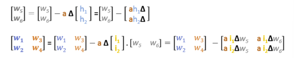
Figure 1: update rules in the neural network
Where a is the learning rate, h1, and h2 are the outputs of the hidden layer, and delta is the difference between the prediction and the actual output.
After the second forward pass, these are the values in the neural network:
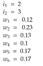
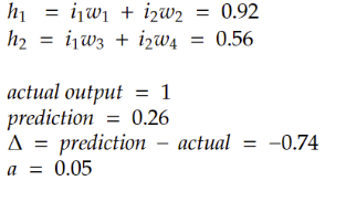
Figure 2: values in the neural network
A backpropagation step would be updating the weights based on the update formula:
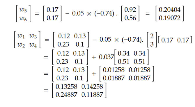
Figure 3: calculations
Based on the new weights, we can calculate the new output of the neural network based on this matrix multiplication in the forward pass:
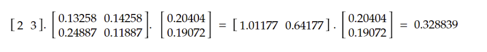
Figure 4: calculations
The forward pass shows that the error is reduced compared to the previous step.
Previous error = 0.26 - 1 = -0.74
New error = 0.328839 - 1 = - 0.671161
This is what we expected. In each step of the gradient descent, we are moving towards minimizing the error function.
Deliverable 2
1. What data augmentation is used in training? Please delete the data augmentation and rerun the code to compare.
Data augmentation is generally used to artificially create more examples and add more variety to the training data by performing random transformations on images, such as rotation, clipping, and scaling. In this notebook, the following techniques are used for augmenting and processing the data:
RandomRotation - randomly rotates the image between (-x, +x) degrees, where we have set x = 5. Note, the fill=(0,) is due to a bug in some versions of torchvision.
RandomCrop - this first adds padding around our image, 2 pixels here, to artificially make it bigger, before taking a random 28x28 square crop of the image.
ToTensor() - this converts the image from a PIL image into a PyTorch tensor.
Normalize - this subtracts the mean and divides by the standard deviations given.
If we delete the data augmentation part, we will have fewer variations in the training samples, which can result in overfitting.
In this notebook, we can comment the following lines in the transforms.Compose() in order to avoid rotation and cropping in the data augmentation. (We still need to keep toTensor() and normalization since they are necessary preprocessing for the data)
train_transforms = transforms.Compose([
#transforms.RandomRotation(5, fill=(0,)),
#transforms.RandomCrop(28, padding=2),
transforms.ToTensor(),
transforms.Normalize(mean=[mean], std=[std])
])
Here are the metrics during the training process with data augmentation:
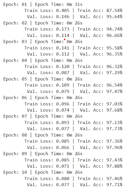
Figure 5: metrics during training procress with data augmentation
Here are the metrics during the training process without data augmentation:
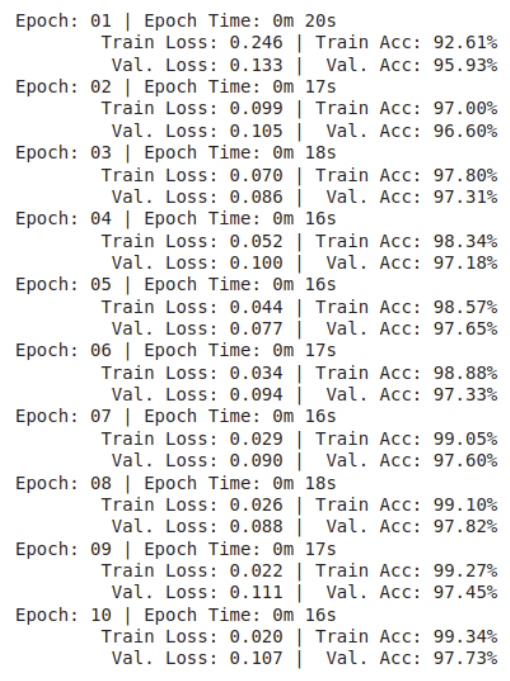
Figure 6: metrics during training procress without data augmentation
(Note: results in each run might slightly differ due to the stochastic nature of the neural networks. However, fixing the seeds(which is done in this notebook) helps to have reproducible results.)
The test accuracy is as follows:
Without data augmentation: 97.91%
With data augmentation: 98.12%
The lower test accuracy in the case without data augmentation is an early sign of overfitting. ( The model has high accuracy on the training set, but low accuracy on unseen data (test set). )
2. What is the batch size in the code? Please change the batch size to 16 and 1024 and explain the variation in results.
The current batch size in the code is 64.
The batch size indicates the number of samples that are processed by the model in each epoch, before updating the model parameters.
A larger batch size can provide a more accurate estimate of the gradient because it is using the information from more data, but it will take longer to converge because it needs more computation in each epoch.
On the other hand, a smaller batch size results in more noise in the gradient since its using the information from a smaller set of data to do the update, but it can lead to faster convergence since it is less computationally expensive.
More generally, “batch size” is a hyperparameter we have to decide, to guarantee the best convergence. We decide the value of the batch size based on the tradeoff we explained above.
In this notebook, if we change the batch size to 16, the training results will be as follows:
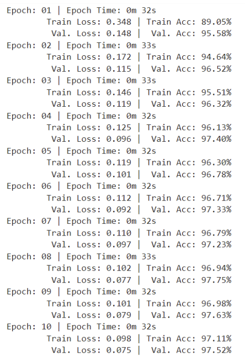
Figure 7: metrics during training procress with batch size of 16
And the test accuracy is 98.13%.
And the results for the batch size of 1024 is:
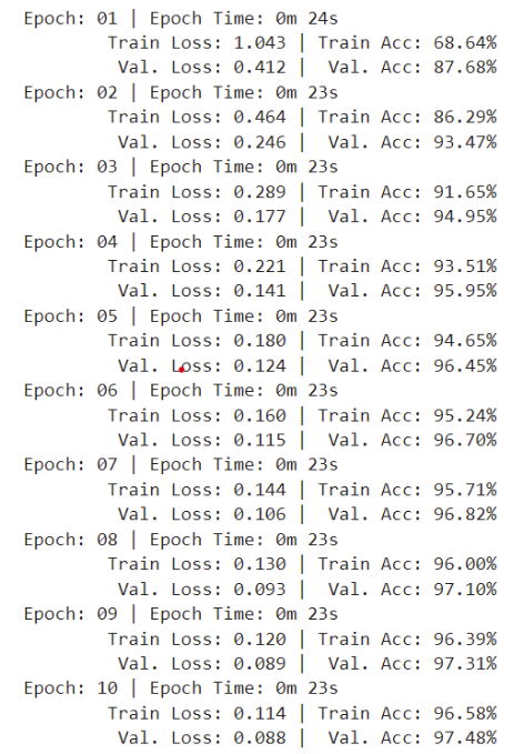
Figure 8: metrics during training procress with batch size of 1024
And the test accuracy is 97.54%
In our case, the smaller batch size works better.
The smaller batch sizes are less stable in general, but they tend to help the network converge to the optima faster.
3. What activation function is used in the hidden layer? Please replace it with the linear activation function and see how the training output differs. Show your results before and after changing the activation function in your written report.
The activation function used in the notebook is ReLU.
The activation function’s job is to add nonlinearity to the output.
If we replace ReLU, with linear activation function,( which is the identity function, or it is just like applying no nonlinearity to the unit output) then the neural network loses its ability to learn complex patterns in the data.
In this notebook, in order to change ReLU to linear activation function, we need to change the forward method in the MLP class as follows:
def forward(self, x):
# x = [batch size, height, width]
batch_size = x.shape[0]
x = x.view(batch_size, -1)
# x = [batch size, height * width]
h_1 = self.input_fc(x)
# h_1 = [batch size, 250]
h_2 = self.hidden_fc(h_1)
# h_2 = [batch size, 100]
y_pred = self.output_fc(h_2)
# y_pred = [batch size, output dim]
return y_pred, h_2
The results after applying linear activation function is as follows:
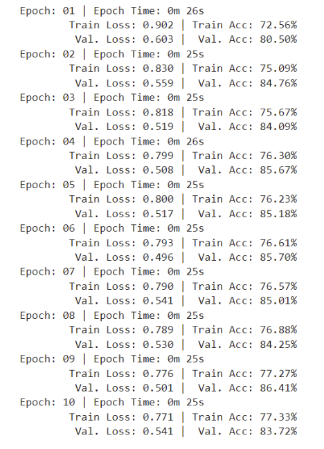
Figure 9: metrics with linear activation
And the test accuracy is 87.02%.
The results for the network with ReLU was shown in earlier figures.
As you can see, changing ReLU to linear activation function causes a sharp decrease in network’s performance.
4. What is the optimization algorithm in the code? Explain the role of the optimization algorithm in the training process
The optimization used in the notebook is “Adam”.
Adam is an adaptive learning rate optimization algorithm that is used in machine learning.
Optimization algorithms use the information we already have about the gradient, to improve the gradient descent update rule, and to make convergence faster.
Some examples of optimization algorithms are AdaDelta, RMSprop, AdaGrad, and Adam.
Adam, for example, is a combination of Momentum and RMSprop.
The momentum algorithm takes into account the “exponentially weighted average” of the gradients in the weight update formula.
The RMSprop is an extension to the AdaGrad optimization algorithm which uses an exponential moving average instead of the cumulative sum of squared gradients in the update rule.
Adding all this information to the update rule, instead of solely updating the weights of the network based on the gradient, can make the convergence faster.
Here is how the weight update rule changes in the Adam optimization algorithm:
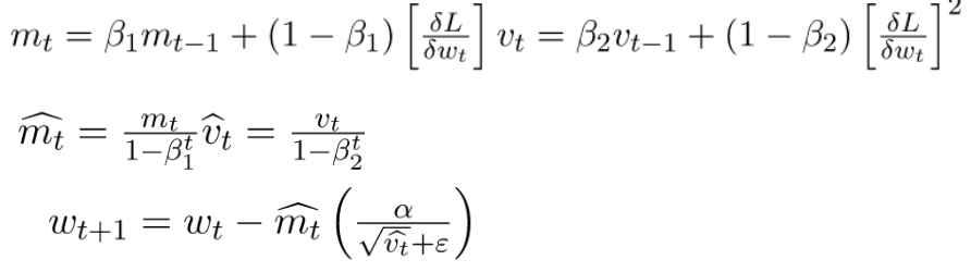
Figure 10: adam optimization update formulas
5. Add dropout in the training and explain how the dropout layer helps in training.
We can add dropout by including a dropout layer in the NN architecture.
The dropout layer works by randomly blocking off a fraction of perceptrons in a layer, during training, and setting their output to zero. This means that the contribution of these switched-off perceptrons to the activation of downstream perceptrons is evacuated on the forward pass., and the model is forced to learn more robust features which are less dependent on specific input features. Dropout is a regularization method that can avoid overfitting. The reason it is effective is that dropout prevents all the perceptrons in a layer from synchronously optimizing their weights. This adaptation prevents all perceptrons from converging to the same goal and decorrelates the weights which can prevent overfitting.
It is usually more common to add dropout to the hidden layers.
In this notebook, we can add dropout by editing the MLP class as follows:
0.2 means the output will be zero with a probability of 0.2.
class MLP(nn.Module):
def __init__(self, input_dim, output_dim):
super().__init__()
self.input_fc = nn.Linear(input_dim, 250)
self.hidden_fc = nn.Linear(250, 100)
self.dropout = nn.Dropout(0.2)
self.output_fc = nn.Linear(100, output_dim)
def forward(self, x):
# x = [batch size, height, width]
batch_size = x.shape[0]
x = x.view(batch_size, -1)
# x = [batch size, height * width]
h_1 =F.relu( self.input_fc(x))
# h_1 = [batch size, 250]
h_2 = F.relu(self.hidden_fc(h_1))
# h_2 = [batch size, 100]
h_3 = self.dropout(h_2)
y_pred = self.output_fc(h_3)
# y_pred = [batch size, output dim]
return y_pred, h_2
The test accuracy is 98.25%, which is higher than our regular network.
We can even further improve the performance by tuning the dropout rate.
Deliverable 3
We discovered that deploying the pytorch model on the robot was not possible due to resource constraints. To fix the issue, we implemented sparse neural networks and backpropagation in C++. Sparse neural networks can achieve strong performance with a fraction of parameters compared to a dense network, and can be deployed in resource constrained settings.
We first tested our implementation on the MNIST dataset and found that it reliably converges to near 100% accuracy on the train set. Due to sparsity, even a small model with 10,000 parameters managed to achieve 96% accuracy on the test set. In comparison, the PyTorch model had 200,000 parameters. We then benchmarked the speed of our code on the jetson nano and found that it can make a prediction in less than 2 ms. The neural network also uses less than 2 MB of memory. The model is so efficient, in-fact, that we can even train it on the duckiebot without any problems.
We first deployed the MNIST pre-trained model on the bot and found that it performed poorly. Our guess is that the distribution shift between the MNIST dataset and the test environment is too large and the model struggles. To fix the problem with the data distribution, we collected a rosbag of data on the bot doing manual control, and trained the model on the data from the duckietown. To get targets (aka labels) for the data, we used the AprilTag IDs. Our final pipeline is as follows:
Detect AprilTags in the image using AprilTag3 library (The C version because we found the Python wrapper to have too much overhead).
Compute and apply a perspective transform on the image using the orientation of AprilTag.
Crop an area above the AprilTag to get the image of the digit.
Our pipeline can very reliably and efficiently detect the location of digits. We feed the image to our implementation of the neural network, which uses a softmax activation to output probabilities over 10 classes. We then compute the target of the image using the ID of AprilTag (Each digit has a unique AprilTag) and update the model parameters to match the target label using gradient descent. Note that we are only using AprilTag for labeling the data, and not for prediction. That means that once the model is trained, the AprilTags can be shuffled and the model would still make accurate predictions.
The complete pipeline, starting from AprilTag detection, computing and applying the perspective transform, digit detection and cropping, model prediction, estimating model gradients using backpropagation, and model update using the Adam optimizer, takes less than 10 ms, making it possible to do learning on the bot at 60hz.
The digit classifier also keeps track of all the digits that have been detected. A digit is considered detected if the last 3 consecutive predictions match. Averaging multiple predictions allows our system to be more robust to occasional classification errors. Once all digits have been detected, the detection node publishes to a node.
A video of the robot running and detecting digits is available here
Lane Following Implementation
Our implementation of lane following is adapted from that in dt-core (code is both borrowed and adapted from this repository). The pipeline summary is as follows:
Retrieve an undistored image from the camera
Detect red, yellow, and white line segments in the image
Project these line segments to the ground plane, enabling localization in the 2D ground frame rather than in the image frame
Using a histogram grid filter, generate an estimate of the Duckiebot’s lane pose consisting of the bot’s offset from the lane centre and the bot’s angle from the lane centre (an angle of 0 here would indicate that the bot proceeds parallel to the lane centre)
Use a PID controller to drive the bot down the lane. The PID controller uses two errors, the bot’s heading and lateral deviation from the lane centre
Linearly decrease velocity and stop at two types of stop lines – the red stop lines in Duckietown and virtual stop lines placed behind other bots
If another bot is in the intersection, then follow it through the intersection. Otherwise, proceed through the intersection in a random direction. Such stochasticity ensures that eventually all digits in this lab will be detected.
After retrieving an undistorted image from the camera, we detect yellow, red, and white contiguous line segments. We do so by first applying Canny edge detection. We then apply a colour filter to select only the red, white, and yellow coloured regions and select only the edges (generated by the Canny edge detection algorithm) in these regions. We then use the Probabilistic Hough Transform to determine the line segments (which consists of a colour, start point, and end point) in each of these regions. We then project each of these line segments to the ground plane using the homography matrix obtained during the extrinsics camera calibration. This allows us to perform lane localization in the 2D ground plane rather than in the image plane.
Next, we generate an estimate of the lane pose of the Duckiebot using a histogram grid filter. We separate the Duckiebot’s lane position and orientation into a grid, and keep a histogram over this grid, outlining our belief of the bot’s true position and orientation in the lane. As the bot moves, we update our belief in the bot’s true lane position and orientation using the belief histogram and the line segments previously extracted. We use the maximum likelihood lane pose in our belief histogram as the prediction of the Duckiebot’s current lane pose.
To follow along lanes, we first retrieve the Duckiebot’s estimated lane pose. We then use a PID controller to adjust the Duckiebot’s driving angle with respect to the lane centre (an angle of 0 indicates the Duckiebot is driving parallel to the lane centre).
The PID controller uses two different targets:
A target angle of 0 with respect to the lane centre
A target offset of 0 from the lane centre
Resulting in two different errors, the Duckiebot’s heading deviation and lateral deviation. The heading deviation ensures that the Duckiebot is driving parallel to the lane centre. The lateral deviation ensures that the Duckiebot is indeed driving down the centre of the lane. We use six hyperparameters for our PID controller (one hyperparameter for each of the proportional, integral, and error terms for each of the two errors). We compute each derivative term using the negative velocity of the Duckiebot’s angle and offset from the lane centre, but our implementation also includes the ability to compute the derivative term using the corresponding errors.
We continuously monitor for stop lines. Upon approaching a stop line, we decrease the Duckiebot’s velocity linearly with the distance to the stop line. Once we reach the stop line, the Duckiebot stops. The linear decrease in velocity can make stopping at the stop line more accurate, which can help with obstacle avoidance. We use two different types of stop lines. First, a node publishes stop lines at the red stop lines at intersections in DuckieTown. Second, an additional node publishes virtual stop lines behind Duckiebots in front of our bot based on the location of the dotted pattern on the back of the front Duckiebot. This implementation allows for significant code reuse.
Once the Duckiebot stops at a red stop line in Duckietown, it decides which direction to proceed through the intersection (note that intersection navigation does not happen at virtual stop lines behind Duckiebots). This direction is uniformly randomly selected from all legal directions through the intersection, indicated by an apriltag at the intersection. By proceeding through the intersection in a random direction, we can ensure that the entirety of Duckietown is eventually visited. For this lab then, we rely on stochasticity to ensure that all digits are eventually seen as the Duckiebot drives autonomously through Duckietown.
To proceed through an intersection, the Duckiebot uses three hyperparameters for each possible direction through the intersection (left, right, straight) for a total of nine hyperparameters which must be manually tuned for each bot. These hyperparameters are the velocity and angular velocity to apply to the bot as well as a specified sleep period.
To proceed through the intersection, the bot first disregards any lane following commands. It then sets its velocity and angular velocity to the corresponding hyperparameters and sleeps for the specified time. For example, when turning left the bot may set its (velocity, angular velocity) = (0.3, 1.3), apply these forces, and sleep for 1.75 seconds. After the sleep time, lane following controls are considered once again. This implementation is similar to that used in dt-core, albeit much simpler.
Other things we tried:
We found the AprilTag detection using Python to be too slow so we first tried detecting digits using image processing. We used the hsv_slider.py file from eclass to find a mask for detecting the background color of the digit, and then used contour detection to detect the digit. The method was not reliable because once in a while, the detector would detect the background pixels as the digit. The neural network classifier, which has not been trained to withhold predictions on random images, would make random predictions on the random images. We realized that for accurate predictions, it’s imperative to detect the digit accurately. Implementing Apriltag detection in C++ turned out to be the most robust and efficient solution.
References
Intuition of Adam Optimizer - GeeksforGeeks
Advantages of the dropout layers - Machine Learning for Developers [Book].